fNIRS analysis
Analysis pipeline
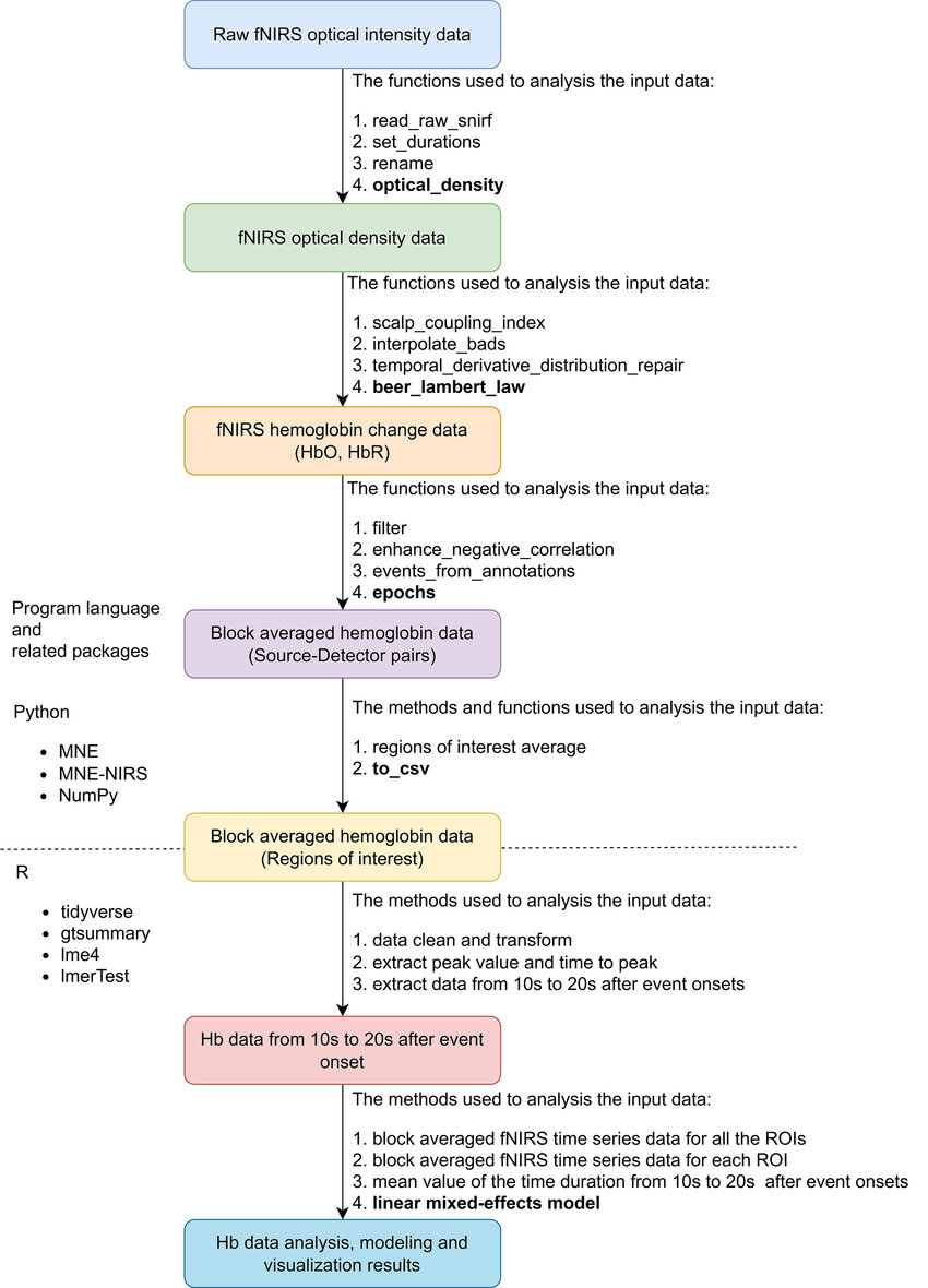
The analysis of fNIRS data involves several key steps that work together to transform raw signals into meaningful insights through statistical analysis. This section outlines the primary components of the pipeline and provides detailed explanations of each stage.
There is no single ‘go to’ solution for the analysis pipeline, always keep in mind that fNIRS is an emerging field. Preprocessing steps can be study- and sample specific (e.g., children vs. adults, computer-based vs. unconstrained interactions).
Preprocessing
Before beginning preprocessing, it is recommended to convert your data into BIDS (Brain Imaging Data Structure) format. This ensures compatibility with various analysis software and facilitates a more standardized pipeline.
Preprocessing is a critical step in preparing fNIRS data for analysis, as it ensures that the data is clean and ready for further statistical analyses. The process begins with a visual signal quality check, where raw fNIRS signals are examined to identify and exclude noisy or corrupted channels based on heart rate peaks and detector saturation. After the visual inspection, in the next step, raw intensity data is converted into optical density, which reflects the changes in attenuation. Then a second automated quality check is carried out based on for instance the scalp coupling index (SCI), which is a measure of the quality of the connection between the optodes and the scalp for each channel. Finally, the optical density data is converted into concentration changes by applying the modified Beer-Lambert law.
Even though fNIRS is less sensitive to external factors, such as moving, the data is not noiseless. To only extract information evoked by the specific task or stimuli, the data needs to be filtered. Different filtering methods are applied to remove systemic physiological noise, such as heart rate, and external factors, e.g., movement artifacts. These artifacts are unrelated to neural activity, thus, can lead to false results. Artifacts can be detected either manually using visual inspection or with automated algorithms. Spontaneous haemodynamic oscillations related to systemic changes are often removed using specific frequency filters. The settings are based on the current experimental design and also the known component frequencies, such as heart rate (~1 Hz), breathing rate (~0.3 Hz), Mayer waves (~0.1 Hz), and very low frequency (< 0.04, VLF) oscillations. In the preprocessing, three different types of filters are applied: high pass filters (removes high frequency components above the cut-off value), low-pass filters (removes low frequency components below the cut-off value), band-pass filters (preserve a frequency range between two cut-off values). Non-systemic artifacts, like movement can be corrected manually or with different algorithms, for instance the temporative derivative distribution repair (TDDR) function.
Read more about the preprocessing steps:
BIDS format for NIRS data
NiReject: toward automated bad channel detection in functional near-infrared spectroscopy
Current Status and Issues Regarding Pre-processing of fNIRS Neuroimaging Data
Comparing different pre-processing routines for infant fNIRS data
Commentary on the statistical properties of noise and its implication on general linear models in functional near-infrared spectroscopy
Temporal Derivative Distribution Repair (TDDR)
Data format and organization by SfNIRS
Automated Processing of fNIRS Data — A Visual Guide to the Pitfalls and Consequences
Annotations, events and epochs
Annotations store time-stamped information about your recorded raw signal data, helping you identify experimental events or conditions. If you are using online triggering during the task, ensure that trigger values align with key experimental events such as stimulus onsets or responses. However, annotations can also be added later based on predefined values or detected artifacts. When manually adding annotations, such as by time frames, make sure that all recording devices operate at the same sampling frequency. For example, if your fNIRS device records at 10 Hz but your online stimulus presentation logging records at 1000 Hz, a direct comparison of event timings without proper synchronization could lead to misaligned annotations. You can make sure that your devices are aligned with proper triggering or using synchronizing software (e.g., LSL).
Trigger values can be renamed to match corresponding conditions or event labels, making it easier to structure your analysis. Annotations are one of the most critical components of functional data recording, as they define events used in data analysis. For the later analysis, multiple annotations can be merged into a single event to allow for different model approaches. Beyond event labeling, annotations can also provide valuable metadata, including markers for noise, motion artifacts, or manual notes indicating segments of data that should be excluded.
Events are special annotations, solely for describing different experimental conditions.
Epochs are representing equal duration chunks of the signal, isolating the data around specific events of interest. Epoching helps to make comparisons across conditions and often used to represent data that is time-locked to repeated experimental events (i.e., block design). To define epochs, time windows are extracted around each event marker, typically ranging from a few seconds before to several seconds after the event. The exact duration of these epochs depends on the task design and the timing of the hemodynamic response. Relative to your event you can easily extract the epochs by defining the required time before (tmin) and after (tmax) the event onset. When creating epochs, you can also decide to reject specific segments of the data based on predefined conditions, e.g., the peak-to-peak channel amplitude.
Not every epoch is evaluated during the statistical analysis. Some epochs can be dropped if it is too close to the start or the end of the recording, so data cannot be averaged for the given timeframe. And epochs can be also excluded automatically or manually based on noise to maintain data quality.
Baseline correction can be applied to these epochs to ensure that the data is normalised relative to a consistent starting point. In the traditional baseline method, you add or substract a scalar amount from every timepoint in an epoch based on the mean signal during the pre-event baseline period, such as -2 to 0 seconds. Choosing the right time window for baseline correction is a question that needs to be decided in the experimental design.
Learn more about annotating and extracting epochs:
Annotating continuous data
Divide continuous data into equally-spaced epochs
Rejecting bad data spans and breaks
GLM vs. Waveform Analysis
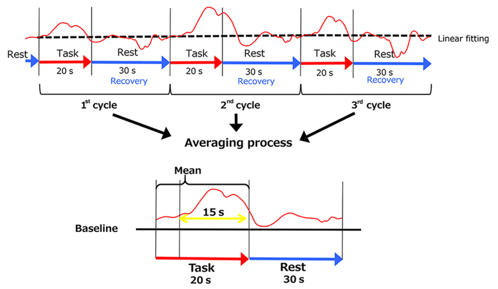
Two primary approaches for analyzing fNIRS data are the General Linear Model (GLM) and waveform analysis. The choice between these methods depends on the specific research question and experimental design. Waveform analysis (block averaging, time-course analysis) focuses on analyzing the raw time-course of signals, examining their shape, amplitude, and timing. This is a simpler and less computationally intensive method, making it useful for exploratory analysis. It involves averaging waveforms across trials for each condition and comparing features such as peak amplitudes, latencies, or areas under the curve between conditions.
Waveform analysis is used when the research question is focusing more on the basic signal characteristic, like peak amplitude. These charachteristics can be evaluated better across a high number of trials (strict block design) and for tasks where strong haemodynamical response is expected (e.g., finger tapping). Moreover, it is easier to interpret the results and visualize with averaged signals. The method can also be used to extract evoked repsonses to implement later in different custom built linear models. Waveform analysis has some limitations, such as being more sensitive to noise and artifacts, as it does not explicitly account for confounding variables.
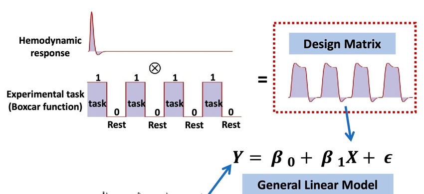
General Linear Model (GLM; similar to SPM approach in different modalities) is used to estimate the relationship between predictors, such as task conditions, and the observed signals. It is often used with more complicated experimental designs (e.g., multiple conditions), in event-related paradigms and in setups where confounding effects are important (e.g., short-distance channels).
It uses a design matrix with predictors (e.g., stimulus onsets) convolved with a HRF to model expected responses. Then the GLM is fitted to the data to extract beta coefficients, which quantify the contribution of each condition to the observed signal for further statistical comparison.
This approach is robust to noise when designed appropriately and can incorporate complex models of neural and physiological processes. GLM also allows for group-level comparisons incorporated in the model. GLM approach is used when testing specific task-related hypothesis in a more complex experimental design (i.e., multiple conditions, covariates or regressors). However, a downside of the GLM approach is that it requires an a priori assumption about the shape of the hemodynamic response, which may not always accurately reflect the actual neural activity. Additionally, it is computationally intensive and sensitive to model specification, making it less suitable for exploratory analyses.
Read more about the analysis methods:
Analysis methods for measuring fNIRS responses generated by a block-design paradigm
Analysis tools
When it comes to analysis tools, there is a broad range of available packages, toolboxes and software that can be used. These involve specific analysis sofware made by the different manufacturers and packages and toolboxes in Python and MATLAB. Automated analysis pipelines can simplify tasks with automation such as applying filters and motion artifact corrections, but also helpful when performing the statistical analyses or generating plots and topographies.
MNE-Python
MNE-Python includes fNIRS-specific modules in the MNE-NIRS package as well as general-purpose data analysis tools like NumPy, SciPy or Matplotlib. It is an open-source package developed primarily for MEG and EEG analysis but also extended with NIRS features in the past years. The package can be installed in a standalone version or via pip or conda for experienced Python users. Another advantage of MNE that you can easily convert your raw data into BIDS structure with the MNE-BIDS package.
With MNE you can carry out an extensive NIRS data analysis pipeline from preprocessing to visualization with many available helps in the documentation and online forums. With different export options it is also possible to carry out your later analysis in different software and only use this package for the neuroimaging data analysis pipeline.
nirsLAB
nirsLAB is a MATLAB-based analysis tool developed specifically for analysing data recorded with NIRx devices, meaning it only works with .nirs datafiles (no support for snirf). The environment has a step-by-step GUI for all the required steps in the analysis pipeline, including the preprocessing and the statistical analysis (SPM). The analysis process allows you to extract event-related activation from the signal time series data. Level 1 focuses on the level of subject, while Level 2 focuses on the group=level.
This software can be highly useful when first working with fNIRS data or if someone wants to analyse NIRS data without coding expertise.
nirsLAB manual with installation guide
MATLAB toolboxes
Many MATLAB-based toolbox exist for analysing fNIRS data, which can be especially useful when integrating fNIRS with different modalities such as EEG or co-registration with structure sensor. On the following links you will find three different packages developed for or compatible with NIRS analysis pipelines.
FieldTrip installation and setting up the path
Learn more about the different analysis software:
fNIRS analysis toolbox series by Artinis
fNIRS analysis guide by NIRx
MNE tutorial by Dr. Robert Luke
Ideas and software for analyizing fNIRS data
Software developed for use in fNIRS imaging by SfNIRS